Gallery: Miscellaneous
Examples
1) dmmaskfill: paint by number
Whether making temperature maps, variability maps, or maps of hardness ratios, it is often convenient to start your analysis with a map that groups pixels together. Typically these maps have integer values where the pixel value identifies group membership. The CIAO tools dmnautilus and dmimgblob both produce such a map as part of their outputs. Examples of these can be seen in the Binning and Detect galleries. There are various other non-CIAO tools that also apply their own grouping scheme and output similar data products.
These maps can be use to select data for analysis for each individual region. Once the analysis is complete -- whether it is computing a temperature, or measure of variability, etc -- it is often helpful to visualize the results by mapping the analysis results back to spatial regions from whence they originated.
This is easy to do with the dmmaskfill tool.

dmimgpick "acisf06934N002_evt2.fits[ccd_id=7,energy=500:3000]" 6934_s3.contour.map 6934.mapped.evt method=closest clob+
dmlist 6934_s3.contour.map data,clean,array  | grep -v ^# | sort -n | uniq > map.dat
cat map.dat | xargs -I@ dmstat "6934.mapped.evt[cols energy][contmap=@]" | grep mean | cut -d: -f2 > mean_energy.dat
dmpaste map.dat"[cols contmap=col1]" mean_energy.dat"[cols energy=col1]" lookup.tab  clob+
dmmaskfill lookup.tab 6934_s3.contour.map 6934_s3.contour_filled.map clob+
The following commands can be used to visualize the output
ds9 6934_s3.contour_filled.map -scale limits 1200 1400 -linear -cmap load $ASCDS_CONTRIB/data/iman.lut -view colorbar yes
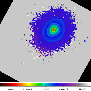
In this example we are going to compute the mean energy for the events in the Abell 2597 cluster. We have used an external package to compute a map, 6934_s3.contour.map, where the pixels have been grouped along various flux contours.
The first step is to identify which events belong to which region. This is easy to do with dmimgpick. This adds a new column to output table which gives the map value which is method=closest to the event location. In this example the new column is called CONTMAP.
The next step is make a table which is a list of all the pixel values in the map. We use dmlist with the data,clean,array options to generate a list of all the pixel values. The header line is removed with the grep -v ^# command. The values are then sorted numerically and the unique values are stored in the file map.dat.
The next command then runs the dmstat command for each unique map value. The UNIX xargs command is a very handy utility to use for this kind of looping. As demonstrated here, xargs takes each line from the map.dat file (via standard input), and runs the dmstat command shown, but replacing the @ with the value on each line; eg if the line is '100' then it runs the command
dmstat "6934.mapped.evt[cols energy][contmap=100]"
The rest of the command then selects the mean output value and stores the results in a file called mean_energy.dat.
We now have one file which contains the map ID number, map.dat, and one file which contains the mean energy for the events closest to that map ID number, mean_energy.dat. Since the CXC Datamodel can read these simple lists as ASCII files, we then just want to combine them together into a single table using the dmpaste tool. To make things a little more clean, we rename the columns on-the-fly to have more descriptive names.
The final step then is to create the output image shown here by using dmmaskfill to replace the map ID number with the mean energy value. The output shows a map of the mean energy (in eV, since those are the units of the Energy column in the event file). The nature of this cool core cluster is the topic of several papers. While this is not a temperature map, it does provide a way to do some preliminary analysis with that ultimate goal in mind.
2) Convert mask to polygon
While working with region maps as shown in the other example is very convenient, there are times when you may need to convert those mapped pixels into standard CIAO regions (typically polygons). This may be needed for things such as computing areas (although there are other ways to compute areas using dmimghist) or just general compatibility with other tools/packages.
In another example we saw how to use dmimglasso to create a polygon. In that example we skipped over the critical step of how to determine the starting x,y location. This may be obvious/trivial when running things interactively, but when trying to script it can be a little tricky.

dmimgthresh 6934_s3.contour.map 33.map cut=33:33 value=0 clob+
dmstat 33.map cen- sig- med- verb=0
punlearn dmcoords
pset dmcoords x=` stk_read_num ")dmstat.out_max_loc" 1 echo+`
pset dmcoords y=` stk_read_num ")dmstat.out_max_loc" 2 echo+`
dmcoords 33.map op=sky verb=0
pset dmimglasso xpos=`pget dmcoords logicalx | awk '{print int($1+0.5)}' `
pset dmimglasso ypos=`pget dmcoords logicaly | awk '{print int($1+0.5)}' `
dmimglasso 33.map 33.lasso low=33 hi=INDEF coord=logical clob+ mode=h
echo "32.5 33.5 yellow" > 33.tag
The following commands can be used to visualize the output
ds9 6934_s3.contour.map -scale log -region width 2 -region 33.lasso -zoom 3 -pan to 4032 3955 physical -cmap tag load 33.tag
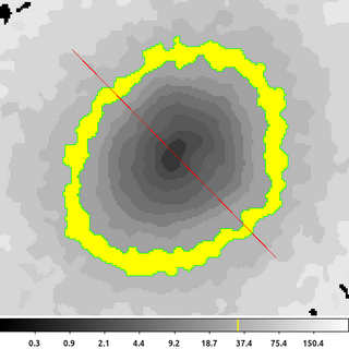
In this example we are going to create a region that encloses map ID 33 in the 6934_s3.contour.map input file. This ID was selected because it corresponds to pixels that form a pseudo-annulus. Therefore, we cannot simply select the center (or centroid) of the image to be the starting point. dmimglasso requires that the starting point be inside the region being created. So we need to identify a pixel (any pixel will do) that is inside the region formed from the map with a pixel value equal to 33.
The first dmimgthresh uses cut=33:33. The cut threshold is implemented such that values strictly less-than 33 are set to 0 and values that are strictly greater-than 33 are also set to 0. This means that only pixels values equal to 33 remain.
The next several commands are used to automatically select the starting point for dmimglasso. We start by running dmstat. In this example, the center/centroid is not useful; however, dmstat also outputs the location of the maximum pixel value: out_max_loc. Since we are using the input that has been run through dmimgthresh, we know that the maximum pixel value for the map ID is 33, which is where we want dmimglasso to start.
Now while it is tempting to take dmstat's out_max_loc value and use that directly, users will find that due to the numerical precision of the output, this will sometimes fail. To make this process robust, we need to convert the out_max_loc location from physical coordinates to integer logical coordinates. This solves the problems with numerical precision and avoids issues dealing with needing to know the image bin size.
We do this by using the stk_read_num tool to parse the dmstat output using the ")" parameter file redirect syntax. dmstat stores the location of the maximum pixel value into the out_max_loc parameter as a comma separated pair of x,y values. stk_read_num is used to read each value: 1 for x, 2 for y. Those values are pset into dmcoords' parameter file.
Then we run dmcoords with op=sky, which uses the values that were just pset. dmcoords converts those sky coordinates to various other Chandra coordinate systems, including the logical (image) coordinates we are looking for.
dmcoords stores the logical coordinates in two parameters: logicalx and logicaly. These values are real-valued. We use the UNIX awk command convert these to integers by rounding them to the closest pixel. These are pset into the dmimglasso parameter file.
Finally, the dmimglasso tool is run. The important thing to note is the use here of coord=logical to let the tool know that the input coordinate are to be interpreted as image/logical pixels.
The final echo is used to create a ds9 Color Tag file which is used to apply a color to range of pixel values. In this case, pixel values between 32.5 and 33.5 will be colored yellow.
The image above shows the output region file. It is composed of two polygons. The inner polygon is excluded from the outer polygon to form the pseudo-annulus we were expecting. The red-slash indicating an excluded region is for the inner polygon. The yellow color-tag file has been applied to highlight the pixel values used to create the region.
3) Skeletonize
In this example we take the Gaussian Gradient Magnitude output and perform further analysis.
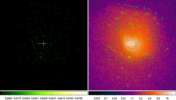
The output from that example shows a sharp edge (large gradient magnitude) to the South-East of the center of the cluster. We can refine the estimate of the location of the edge by applying a skeletonization technique.

dmimgfilt abell496_ggm.img ggm_h.img function=peak mask="box(0,0,1,3)" clob+
dmimgfilt abell496_ggm.img ggm_v.img function=peak mask="box(0,0,3,1)" clob+
dmimgfilt ggm_h.img,ggm_v.img ggm_skel.img function=max mask="box(0,0,3,3)" clob+
dmimgthresh ggm_skel.img - cut=INDEF value=0 | dmimgthresh - ggm_skel_thresh.img cut=0.002 value=0 clob+
The following commands can be used to visualize the output
ds9 ggm_skel_thresh.img abell496_broad_thresh.img -frame 1 -pan to 4065 3890 physical -cmap load $ASCDS_CONTRIB/data/green8.lut -frame 2 -scale log \
    -smooth -pan to 4065 3890 physical -cmap load $ASCDS_CONTRIB/data/gem-256.lut -mask color green -mask transparency 0.5 -mask ggm_skel_thresh.img \
    -pan to 4065 3890 physical
The GGM is the magnitude of the gradient (after being smoothed with a Gaussian). We can define the location of an edge to be where the magnitude of the gradient is maximum.
The first two runs of dmimgfilt with function=peak decomposes the GGM image into horizontal and vertical edges. The peak statistic is used to search for the local maximum in a vertical (1x3) and horizontal (3x1) box. The peak function returns the current pixel value if it is the maximum value of the pixels in the mask; if the current pixel is not the local maximum then the output pixel is set to NaN.
We then combine the horizontal and vertical edges together. The dmimgfilt tool is used again, but this time with a stack of inputs: the horizontal and vertical edges, and now using the max function. The output then is the maximum pixel value in a sliding 3x3 box taken from either of the two input files. If the edge is not detected in either input, the output will be NaN. If the edge is detected horizontally, that value is used. If the edge is detected vertically, that value is used. If both, then the maximum value is used (which in this case will be the same in each dataset).
The output skeleton image then contains either the GGM pixel value if that pixel was detected as the local maximum in either the horizontal or vertical direction, or NaN if not. Since the majority of the pixels are not local maxima, most of the output pixels are NaN.
We then apply two separate thresholds to the pixel values. First, pixel values set to NaN are replaced with 0. This makes displaying the dataset easier. Then we apply an adhoc lower level threshold of 0.002. This value was selected for this example dataset based on trial and error to reduce appearance of edges due to random background fluctuations.
The image on the left is the skeletonized GGM. The pixel values are equal to the pixel values in the GGM image where the gradient magnitude is maximum.
The image on the right shows the original data with the skeletonized GGM overlaid on top as a ds9 mask.
This type of output is not necessarily intended to represent a final data product. It is intended to help assist users in locating interesting spatial regions to perform additional data analysis.