Gallery: Detect
Examples
- Source Detect Regions: wavdetect
- Source Detect Regions: celldetect
- Source Detect Regions: vtpdetect
- Pseudo detect: get_src_region
- Connected pixels: dmimgblob
1) Source Detect Regions: wavdetect
wavdetect is the most popular CIAO source detection tool. It detects sources by convolving the input image with a Haar wavelet (aka Mexican Hat wavelet). The negative part of the outer annulus provides a natural local background subtraction and the Gaussian like central peak acts like a matched-filter.
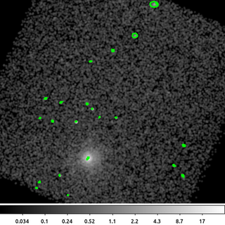
pset wavdetect infile=acisf00578_s3_broad.img
pset wavdetect outfile=wav.src
pset wavdetect psffile=acisf00578_s3_broad.psfmap
pset wavdetect expfile=acisf00578_s3_broad.expmap
pset wavdetect scellfile=wav.cell
pset wavdetect imagefile=wav.recon
pset wavdetect defnbkgfile=wav.bkg
pset wavdetect scales="1.4 2 4 8 12 16"
pset wavdetect clobber=yes
wavdetect mode=h
The following commands can be used to visualize the output
ds9 acisf00578_s3_broad.img -region wav.src -scale log -block 2 -cmap grey -smooth -regions select all -regions width 3 -region select none
The output source list from wavdetect is a FITS region file that can be directly displayed with ds9. The ellipses show the size of the detected source.
It is important to remember that the output from wavdetect are candidate source detections based on the inputs provided. Users should carefully scrutinize the output list. Also remember that wavdetect is not a photometric tool. While it does provide an estimate of the net source counts, users will want to use more advanced tools such as srcflux to determine fluxes.
2) Source Detect Regions: celldetect
celldetect is a classic sliding-cell detection algorithm. It computes the SNR for pixel values inside a square compared to the local background sampled from a 1 pixel outer box-annulus. The cell size is adjusted to match the size of the PSF making it optimized for detection of point sources.
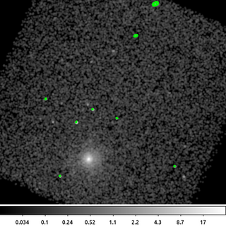
celldetect acisf00578_s3_broad.img cell.src psffile=acisf00578_s3_broad.psfmap expstk=acisf00578_s3_broad.expmap clob+
The following commands can be used to visualize the output
ds9 acisf00578_s3_broad.img -region cell.src -scale log -block 2 -cmap grey -smooth -regions select all -regions width 3 -region select none
The celldetect output is similar to the wavdetect output; however, some bright, off-axis sources are missed. This may be due to the default SNR thresh=3 or may be due to the sources being sufficiently large compared to the PSF calibration.
Since celldetect runs so quickly, it is easy for users to experiment with different parameters settings.
3) Source Detect Regions: vtpdetect
Both celldetect and wavdetect work by looking for sources of certain spatial sizes (celldetect cell size or wavdetect wavelet scales). The vtpdetect tool is completely different. It works by computing the Voronoi Tessellation of the input image. The area of each cell is then used to compute a surface brightness density histogram (counts per area). This histogram is compared to the expected histogram for a flat Poisson background. A source threshold is established from where these curves diverge; those cells are then grouped together to create sources. Since the algorithm doesn't make any assumptions about a source's size or morphology, it can detect arbitrary, extended objects.
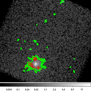
vtpdetect acisf00578_s3_broad.img outfile=vtp.src expfile=acisf00578_s3_broad.expmap clob+ mode=h
The following commands can be used to visualize the output
ds9 acisf00578_s3_broad.img -region vtp.src"[src_region]" -scale log -block 2 -cmap grey -smooth -regions select all -regions width 3 -region select \
    none
The vtpdetect output source list contains two FITS extensions. The first block contains source ellipses and properties very similar to celldetect and wavdetect. The ellipses are computed from the second order moments of the data and are representative of the source size. The second block contains the actual polygons based on the tessellation.
As this example shows, vtpdetect easily detects the extended emission in this dataset. The source polygon in this case is very complicated. Not only is the exterior outline very irregular, but the polygon actually has holes in which are shown as excluded regions (red slash through them).
It can be useful to display these polygons, especially if the first block contains thin/narrow ellipses.
4) Pseudo detect: get_src_region
get_src_region works by computing the histogram of the pixel values in the input image, using the mean and standard deviation of this histogram to set a source pixel threshold, and then grouping all the source pixels together.
The unusual thing about this tool is how it groups source pixels together. Rather than trying to identify sources as sources, it just identifies regions where the pixels are above the background. It uses a series of rectangles to identify these regions without ever trying to associate the pixels with any specific source.
This tool can be used to quickly exclude sources from the background (or could for example be used to exclude point sources on top of extended emission).
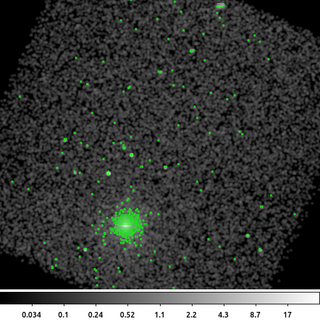
dmimghull acisf00578_s3_broad.img acisf00578_s3.fov clob+
get_src_region "acisf00578_s3_broad.img[sky=region(acisf00578_s3.fov)][bin sky=4]" outfile=gsr.src invert+ clob+ mode=h
The following commands can be used to visualize the output
ds9 acisf00578_s3_broad.img -region gsr.src -scale log -block 2 -cmap grey -smooth
Since get_src_region computes a histogram of the pixels in the image, we need to be sure that we let it know which pixels in the image are exposed. So the first thing we do in this example is use dmimghull to create a pseudo field-of-view (FOV) region file. This is simply a convex polygon that encloses all the non-zero pixels in the image.
Now when we filter with region, the get_src_region tool will know that the pixel values equal to zero in the corners of the image should not be included in this histogram (and therefore will not skew the results).
In this example we inverted the region logic, invert+, which outputs included rectangles. The default is to output a region where the rectangles are excluded.
5) Connected pixels: dmimgblob
It is also possible to construct your own source detection algorithm using individual CIAO tools. What all the source detection algorithms basically do is group together pixels with flux above the background. The details are in how the background is determine and where to set the source threshold.
This example shows a simple, home-grown, source detection algorithm.
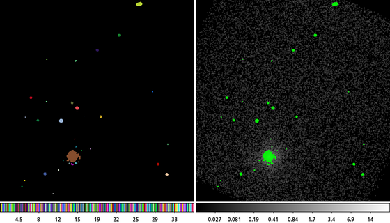
The following commands can be used to visualize the output
ds9 blobs.img acisf00578_s3_broad.img -frame 1 -nan black -zoom 0.5 -cmap load  $ASCDS_CONTRIB/data/005-random.lut  -frame 2 -scale log -zoom 0.5 \
    -cmap grey -smooth  -mask mark range -mask range 0.1 9999 -mask color green -mask transparency 10 -mask blobs.img -frame 1 -view colorbar yes
First, the input image is smoothed with a 3-pixel Gaussian using aconvolve. This not only suppresses noise, but also works as a matched-filter. We only need to remember that convolution and correlation are the same when working with real-valued, symmetrical convolution kernels. Instead of thinking of this as a smoothed image, we can also accurately describe this aconvolve output as the correlation of the input with a 3-pixel Gaussian which emphasizes sources at that same spatial extent.
Next we need an estimate of the background. We use the dmimgfilt median ring technique described in the An Estimated Background Image thread which estimates the background from an median image values in an annulus around each pixel.
dmimgcalc is then used to subtract the background. Since the background was estimated from the same image, there is no need to do any renormalization.
Finally, dmimgblob is used to identify groups of pixels above the threshold. In this example, we selected thresh=0.1 which is 0.1 counts/pixel above the estimated background.
The dmimgblob output is an image whose pixel values identify which group each pixel belongs to. (Left) shows the blob ID numbers. Each set of connected pixels gets its own ID which have been randomly color coded. (Right) shows the counts data with the blobs overlaid as a mask.