Why? Radial Profile Aperture Corrections

A radial profile is a type of histogram typically created by binning data (ie counts) in a set of (usually) concentric circular or elliptical annuli. There is an assumption that the data in each bin are statistically independent and often the radii are chosen to be larger than the PSF to establish independence. However, given the variability in the size and morphology of the PSF this assumption of independence is rarely, if ever, strictly true. That is, the observed counts in any annulus contains a contribution from neighboring annuli.

In this Why? topic we look at

1. A way to estimate the aperture correction needed to apply to each annular bin to account for contributions by neighboring bins.
2. A way to include this aperture correction when modeling the radial profile and how it can affect fit parameters

See Also:

• mkrprm help file.

Example

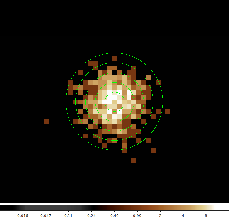
As an example we have simulated a 2D Gaussian with sigma=3 pixel (FWHM=7.1 pixels) and convolved it with the Chandra PSF using marx. The center of the Gaussian is 0.22 arcmin off axis. We generated radial profile bins going from 0 to 10 pixels in steps of 2 pixels (so ~1 arcsec wide each). No background was included in the simulation. The dataset looks like:

What we want to know is the contribution of the source counts from each annulus to each of the neighboring annuli. We will use a Gaussian function to approximate the Chandra PSF since the PSF cannot be modeled analytically. The basic steps are:

• Create a map/mask of each annulus. Pixels inside the annulus are set to 1. Pixels outside the annulus are set to 0.
• Normalize the map so that the pixels sum to 1.0 by dividing by the number of pixels inside the annulus.
• Following the PSF Size Image Smoothing thread we adaptively smooth the normalized map with a Gaussian. The size of the Gaussian is determined by running the mkpsfmap tool with units=logical and using dmimgadapt to perform the smoothing.
• Now for each non-normalized map, we multiply the adaptively smoothed image with the map and compute the sum of all the pixel values. This gives us the approximate contribution of the fraction of the source counts in each annulus from each neighboring annulus.

These steps have been automated in the mkrprm script.

We can see that this is an O(N²) operations since for each input radial bin (ie annulus) we have to loop over all radial bins. The following image illustrates how this comes together.

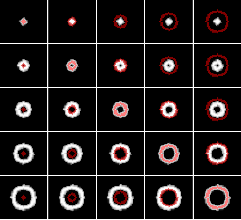
Each row here represents each annulus adaptively smoothed with the Gaussian approximation to the PSF shown as grey scale pixels. Each column in each row shows each of the 5 annuli shown as a transparent red mask. In the top row, left column we see that the smoothed data extends beyond inner most annulus and that is collected in the second annulus. Similarly in the second row, second column, we see that most of the PSF smoothed area is collected in the second annulus, but there is some fraction of the smoothed data that are imaged in both the first and the third annuli. And so on.

Taking it a step further we can then display the fraction of PSF smoothed annulus in each annular bin as a 2D image. Note: The Y-axis has been flipped to match the previous image.

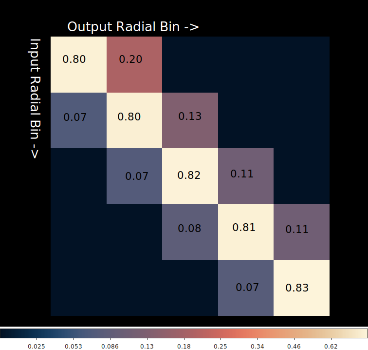
The result is a nearly diagonal matrix. This is to be expected since we are expecting that majority of each PSF smoothed annulus will be imaged in that bin with a smaller fraction imaged in neighboring bins. The values shown are the fraction in each input vs. output bin combination. Note that the each row sums to a total of 1.0; that is all the area is imaged in some annulus except for the last row which has a total of 0.90 which indicates that 10% of the last annulus bin extends beyond our last annulus.

This is the radial profile aperture correction matrix. It does not matter if the regions are circular, elliptical, or even if they are co-located at the same coordinates.

Applying Radial Profile Aperture Correction Matrix

The radial profile aperture correction matrix is very similar to the standard Redistribution Matrix Function/File (RMF) used when doing spectral fitting. The spectral RMF provides the mapping from input Energy (on some grid) to observed Pulse Height (on some different grid). The radial profile response matrix provides the mapping from input annulus to output annulus.

Unfortunately the same RMF models cannot be used with fitting radial profiles. There are a lot of assumptions and requirements built into how RMF files are handled that are not appropriate when fitting radial profile data. Therefore a new generic MatrixModel has been added to the CIAO contributed scripts package that will allow the user to include a matrix multiplication (ie convolution) when modeling their dataset.

First we extract the radial profile from the simulated image. Reminder that the input to the simulation was a Gaussian with FWHM=7.1 pixels.

dmextract "simul.img[bin sky=@ciao.reg]" radial.prof op=generic error=gehrels clob+

and compute the radial profile response matrix

mkrprm infile=simul.img region=@ciao.reg outfile=out.matrix

Next we fit the radial profile using sherpa without including the radial profile response matrix

sherpa> import matplotlib.pylab as plt
sherpa> load_data(1, "radial.prof", 3, ["rmid","sur_bri","sur_bri_err"])
sherpa> set_source(gauss1d.g1)
sherpa> g1.fwhm.min=0.1
sherpa> g1.fwhm.max=20
sherpa> g1.pos.min=-10
sherpa> g1.pos.max=10
sherpa> g1.ampl.min=0
sherpa> g1.ampl.max=100
sherpa> set_method("moncar")
sherpa> fit()
Dataset               = 1
Method                = moncar
Statistic             = chi2
Initial fit statistic = 715.78
Final fit statistic   = 2.50344e-06 at function evaluation 2221
Data points           = 5
Degrees of freedom    = 2
Probability [Q-value] = 0.999999
Reduced statistic     = 1.25172e-06
Change in statistic   = 715.78
   g1.fwhm        7.27827     
   g1.pos         0.252783    
   g1.ampl        0.015377
sherpa> plot_fit_delchi()
sherpa> plt.show()

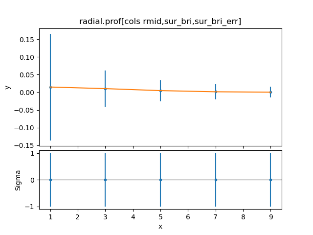
We see that without the radial profile response the fitted value for the FWHM is actually very close to the expected value of 7.1. Unfortunately with only 5 bin and 2 degrees of freedom, it is difficult to get good estimates of the uncertainties.

Next we repeat the fit but this time we include the radial profile response matrix using the MatrixModel.

sherpa> import matplotlib.pylab as plt
sherpa> from matrix_model import MatrixModel
sherpa> from pycrates import read_file
sherpa> load_data(1, "radial.prof", 3, ["rmid","sur_bri","sur_bri_err"])
sherpa> xvals = get_data().x

sherpa> my_file = read_file("out.matrix")
sherpa> matrix = my_file.get_image().values
sherpa> rprof_matrix = MatrixModel(matrix, xvals)
sherpa> set_source(rprof_matrix(gauss1d.g1))

sherpa> g1.fwhm.min=0.1
sherpa> g1.fwhm.max=20
sherpa> g1.pos.min=-10
sherpa> g1.pos.max=10
sherpa> g1.ampl.min=0
sherpa> g1.ampl.max=100
sherpa> set_method("moncar")
sherpa> fit()
Dataset               = 1
Method                = moncar
Statistic             = chi2
Initial fit statistic = 699.153
Final fit statistic   = 2.68446e-06 at function evaluation 1354
Data points           = 5
Degrees of freedom    = 2
Probability [Q-value] = 0.999999
Reduced statistic     = 1.34223e-06
Change in statistic   = 699.153
   g1.fwhm        6.97289     
   g1.pos         0.296586    
   g1.ampl        0.0163763   
sherpa> plot_fit_delchi()
sherpa> plt.show()

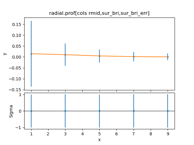
In this case the fit looks nearly identical however the fitted FWHM has now decreased slightly. This is expected. The response matrix essentially blurs the source model to account for the aperture correction needed between neighboring radial profile bins. While the fit without the radial profile response matrix over estimated the FWHM, the fit with the radial profile response matrix under estimates it. This is most likely due the fact that the Chandra PSF is not really shaped like a Gaussian (even this close to optical axis).

Example 2

While the previous example shows some improvement in the estimated fitted value for the FWHM of the simulated dataset; it is a single realization and was chosen with a small number of radii to make it easier to explain. In this example we will use a simulated dataset that has more annuli and repeat the simulation multiple times to look for statistically significant changes to the fitted values.

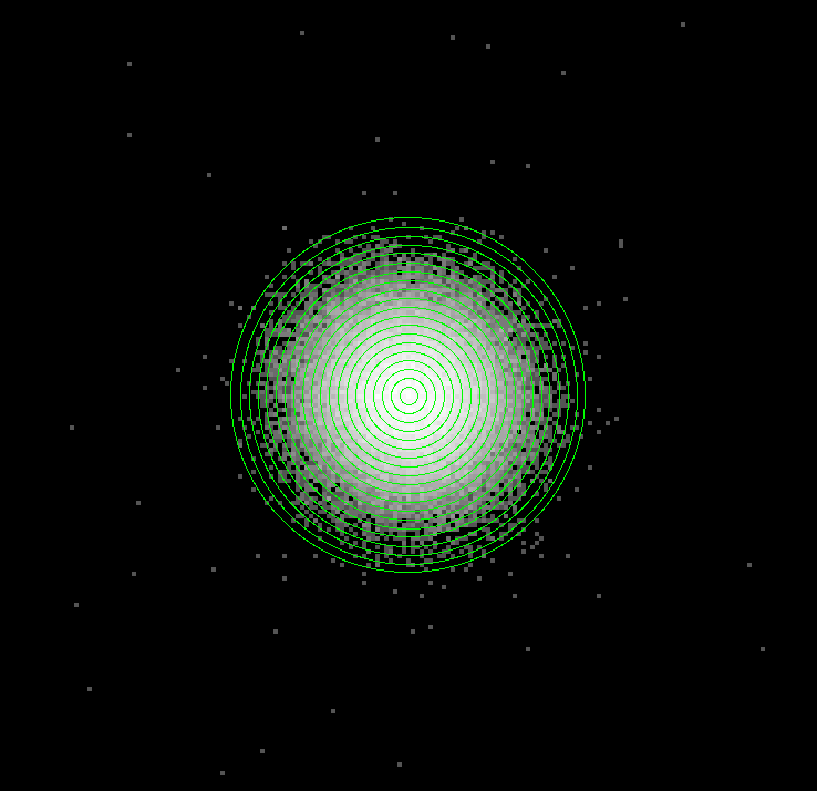
For this example we will use a location that is 5 arcmin off-axis. We still use a Gaussian as the input model but now with a sigma of 10 pixels giving us a FWHM of 23.55. For the annuli we keep the 2 pixel (~1 arcsec) spacing but now include 20 annuli. The simulated image is then run through marx to include the PSF effects. An example simulated image is shown below:

This is one realization of the simulated data with the annulii

Next we compute the radial profile response matrix as before

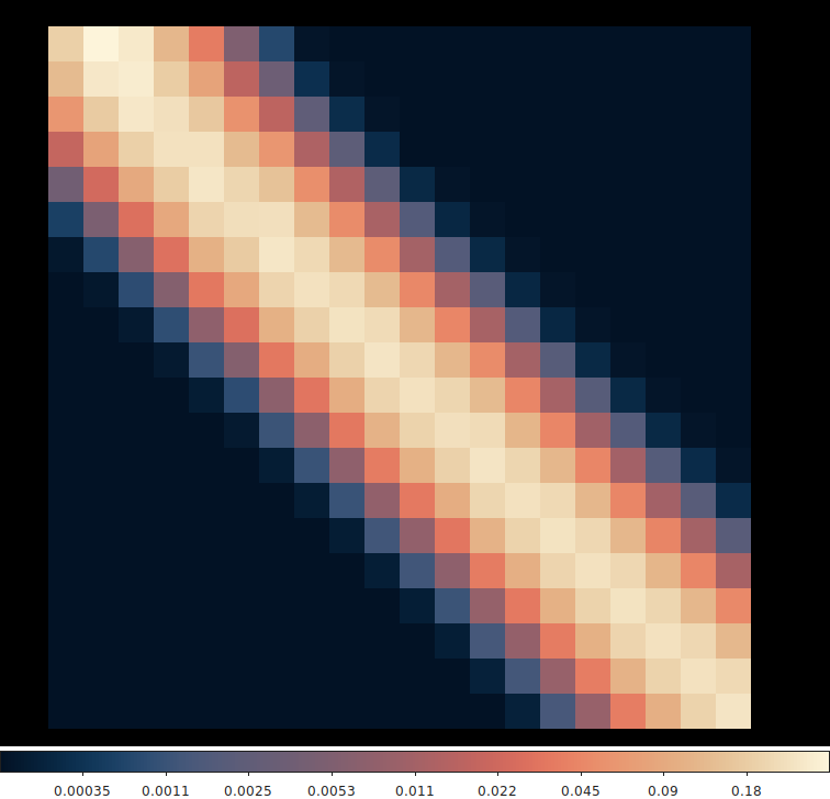
The first obvious difference from before is that being 5 arcmin off axis and keeping 2 pixel (~1 arcsec) radial bins means that the PSF contribution extends into more neighboring pixels. Carefully inspecting the first row (ie inner most radius) we see that that the maximum in that row is in the second column, not the first. The PSF contribution from the inner annulus is actually higher in the second annulus. Why? The choice of radial bin sizes. In this example we have clearly violated the assumption of independence by choosing an 2 pixel wide annulus when the PSF this far off axis is much larger (FWHM ~7 pixels). Since the PSF is so broad and since the second annulus has more area (more pixels) it accumulates more of the total PSF fraction. This somewhat of an extreme example but demonstrates the point that seemingly reasonable bins may not actually be independent.

As before we have fit the data with sherpa using a source model that first omits the radial response matrix, and then again including the radial response matrix. Reminder that we have increased the Gaussian sigma to 10 pixels so we are expecting to get a FWHM of 23.55 pixels. We repeated the simulation 1000 times. We then compare the FWHM fitted without the radial profile response matrix and the FWHM fitted with the radial profile response matrix.

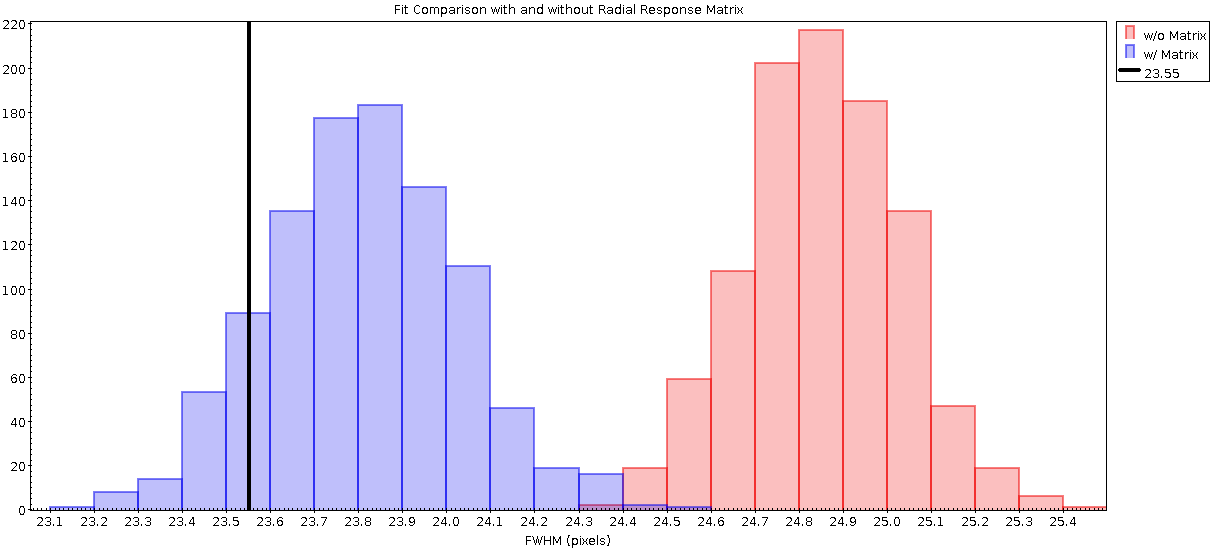
In this figure the red histogram shows the fitted FWHM values without including the response matrix. The blue histogram shows the fitted FWHM values including the response matrix. The solid vertical black line is at the expected/input value of 23.55 pixels. We can see that by including the radial profile response matrix we do get fitted values that are closer to the expected value. However, it's strongly worth noting that the fitted values without including the response pretty good to start with; the mean difference is only off by about 5%.

Summary

In this Why topic we introduced the idea of needing to account for an aperture correction when creating radial profile. Most users try to create statistically independent radial bins to avoid dealing with aperture corrections however that is rarely, if ever, strictly realized. This Why topic discusses how to approximate the aperture correction in the form of creating a radial profile response matrix and how to include it when modeling and fitting.

Analyzing simulated data sets with known model parameters we can see that including the radial profile response matrix does generally improves the estimate of the fitted width of the data; however, it is also true that omitting the radial profile response matrix also yields reasonably accurate fits.