Generation of LSF Reference Data
| Introduction |
| >LSF Reference Data |
| Building LSFPARMS |
| Caveats |
| Validation |
| Summary |
| Other Links |
| isis |
| mit/cxc |
| ciao |
| caldb |
Line Spread Function
We use the term ``Line Spread Function'' (LSF) to describe the redistribution of photons from a source which is a delta function, spectrally and spatially, and integrated in either the dispersion or cross-dispersion direction. The product calculated here by marx includes the HRMA and the grating models, but does not include aspect or pixel randomization effects (these effects are added later in the processing).In flight, the spectra of celestial sources has contributions from several soures which affect the LSF. The most important is the blurring introduced by the mirror (the HRMA PSF) and is discussed in HRMA Calibration document (TBD by HRMA Cal Group). The HRMA PSF is further blurred by the redistribution from the transmission gratings. Additional blurrings are introduced from errors in the aspect solution and pixelation of the detector.
Simulations
The marx provides the calibration model for Chandra gratings. The LSF's are generated using marx 4.0.3 and the internal MARX HRMA mirror model as well as the model for the HETG or LETG to describe the redistribution of photons from a point source. The input parameters for the simulations are chosen to be the nominal set of input parameters; hence the output may not reflect any calibration uncertainties. While the MARX mirror model may not reproduce all the features contained in the more detailed SAOsac raytrace model (via ChaRT interface), it does include all the important effects for integrated properties and gives an excellent description (see marx manual TBD).Generation of the LSF library and RMFs
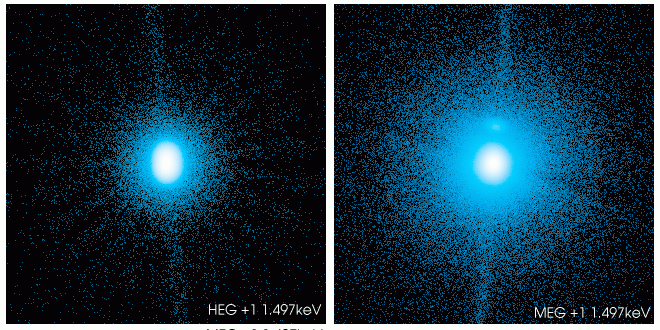
The LSF products are generated from MARX simulations that are run for the on-axis location and contain 500,000 -- 2,500,000 counts per +1 order for each monoenegetic simulation. The raw binary MARX data files are read into IDL and a square region 13''.2 x 13''.2, centered on the centroid position of the monoenergetic line and with 2 micron bin-size (~0.08'') is extracted to make a 2-D histogram. The extracted histogram is also rotated so that its row and column linearly correspond to the grating coordinate system TG_R and TG_D. This histogram is then integrated in the dispersion or cross-dispersion direction to obtain the LSF or the cross-dispersion profile. Figure 1 shows the examples of the extracted 2-D LSF histogram.

The current version of the RMF generation program (e.g., mkgrmf for CIAO) for grating RMFs can produce RMF from a series of simple mathematical functions. To accomodate this the LSF data are fit with two Gaussian and two Lorentzian functions. These fitted functions are then used to construct the HEG and MEG RMFs (LEG not available yet with CALDB 2.17). The cross-dispersion profiles are numerically integrated to derive encircled energy fraction (EE_FRACS), which would also be stored in the LSF library and would be used to normalize the RMFs.
The next section describes how to define LSF and compiled as useful calibration products for CALDB in more details.
| Previous: Introduction | Next: LSFPARMS library |